Slides for this module can be seen
here.
You do not have to look at them before the lecture!
8 Dynamic programming
The term Dynamic Programming (DP) refers to a collection of algorithms that can be used to compute optimal policies of a model with full information about the dynamics, e.g. a Markov Decision Process (MDP). A DP model must satisfy the principle of optimality. That is, an optimal policy must consist for optimal sub-polices or alternatively the optimal value function in a state can be calculated using optimal value functions in future states. This is indeed what is described with the Bellman optimality equations.
DP do both policy evaluation (prediction) and control. Policy evaluation give us the value function \(v_\pi\) given a policy \(\pi\). Control refer to finding the best policy or optimizing the value function. This can be done using the Bellman optimality equations.
Two main problems arise with DP. First, often we do not have full information about the MDP model, e.g. the rewards or transition probabilities are unknown. Second, we need to calculate the value function in all states using the rewards, actions, and transition probabilities. Hence, using DP may be computationally expensive if we have a large number of states and actions.
Note the term programming in DP have nothing to do with a computer program but comes from that the mathematical model is called a “program”.
8.1 Learning outcomes
By the end of this module, you are expected to:
- Describe the distinction between policy evaluation and control.
- Identify when DP can be applied, as well as its limitations.
- Explain and apply iterative policy evaluation for estimating state-values given a policy.
- Interpret the policy improvement theorem.
- Explain and apply policy iteration for finding an optimal policy.
- Explain and apply value iteration for finding an optimal policy.
- Describe the ideas behind generalized policy iteration.
- Interpret the distinction between synchronous and asynchronous dynamic programming methods.
The learning outcomes relate to the overall learning goals number 2, 4, 6, 7, 8, 10 and 12 of the course.
8.2 Textbook readings
For this module, you will need to read Chapter 4-4.7 in Sutton and Barto (2018). Read it before continuing this module. A summary of the book notation can be seen here.
8.3 Policy evaluation
The state-value function can be represented using the Bellman equation Equation 7.2: \[ v_\pi(s) = \sum_{a \in \mathcal{A}}\pi(a | s)\left( r(s,a) + \gamma\sum_{s' \in \mathcal{S}} p(s' | s, a) v_\pi(s')\right). \tag{8.1}\]
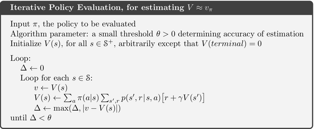
If the dynamics are known perfectly, this becomes a system of \(|\mathcal{S}|\) simultaneous linear equations in \(|\mathcal{S}|\) unknowns \(v_\pi(s), s \in \mathcal{S}\). This linear system can be solved using e.g. some software. However, inverting the matrix can be computationally expensive for a large state space. Instead we consider an iterative method and a sequence of value function approximations \(v_0, v_1, v_2, \ldots\), with initial approximation \(v_0\) chosen arbitrarily e.g. \(v_0(s) = 0 \: \forall s\) (ensuring terminal state = 0). We can use a sweep with the Bellman equation to update the values:
\[\begin{equation} v_{k+1}(s) = \sum_{a \in \mathcal{A}}\pi(a | s)\left( r(s,a) + \gamma\sum_{s' \in \mathcal{S}} p(s' | s, a) v_k(s')\right) \end{equation}\]
We call this update an expected update because it is based on the expectation over all possible next states, rather than a sample of reward from the next state. This update will converge to \(v_\pi\) after a number of sweeps of the state-space. Since we do not want an infinite number of sweeps we introduce a threshold \(\theta\) (see Fig. 8.1). Note the algorithm uses two arrays to maintain the state-value (\(v\) and \(V\)). Alternatively, a single array could be used that update values in place, i.e. \(V\) is used in place of \(v\). Hence, state-values are updated faster.
8.4 Policy Improvement
From the Bellman optimality equation Equation 7.4 we have
\[ \begin{align} \pi_*(s) &= \arg\max_{a \in \mathcal{A}} q_*(s, a) \\ &= \arg\max_{a \in \mathcal{A}} \left(r(s,a) + \gamma\sum_{s' \in \mathcal{S}} p(s' | s, a) v_*(s')\right). \end{align} \tag{8.2}\] That is, a deterministic optimal policy can be found by choosing greedy the best action given the optimal value function. If we apply this greed action selection to the value function for a policy \(\pi\) and pick the action with most \(q\): \[ \begin{align} \pi'(s) &= \arg\max_{a \in \mathcal{A}} q_\pi(s, a) \\ &= \arg\max_{a \in \mathcal{A}} \left(r(s,a) + \gamma\sum_{s' \in \mathcal{S}} p(s' | s, a) v_\pi(s')\right), \end{align} \tag{8.3}\] then \[ q_\pi(s, \pi'(s)) \geq q_\pi(s, \pi(s)) = v_\pi(s) \quad \forall s \in \mathcal{S}. \] Note if \(\pi'(s) = \pi(s), \forall s\in\mathcal{S}\) then the Bellman optimality equation Equation 7.4 holds and \(\pi\) must be optimal; Otherwise, \[ \begin{align} v_\pi(s) &\leq q_\pi(s, \pi'(s)) = \mathbb{E}_{\pi'}[R_{t+1} + \gamma v_\pi(S_{t+1}) | S_t = s] \\ &\leq \mathbb{E}_{\pi'}[R_{t+1} + \gamma q_\pi(S_{t+1}, \pi'(S_{t+1})) | S_t = s] \\ &\leq \mathbb{E}_{\pi'}[R_{t+1} + \gamma (R_{t+2} + \gamma^2 v_\pi(S_{t+2})) | S_t = s] \\ &\leq \mathbb{E}_{\pi'}[R_{t+1} + \gamma R_{t+2} + \gamma^2 q_\pi(S_{t+2}, \pi'(S_{t+2})) | S_t = s] \\ &\leq \mathbb{E}_{\pi'}[R_{t+1} + \gamma R_{t+2} + \gamma^2 R_{t+3} + ...)) | S_t = s] \\ &= v_{\pi'}(s), \end{align} \] That is, policy \(\pi'\) is strictly better than policy \(\pi\) since there is at least one state \(s\) for which \(v_{\pi'}(s) > v_\pi(s)\). We can formalize the above deductions in a theorem.
Let \(\pi\), \(\pi'\) be any pair of deterministic policies, such that \[\begin{equation} q_\pi(s, \pi'(s)) \geq v_\pi(s) \quad \forall s \in \mathcal{S}. \end{equation}\] That is, \(\pi'\) is as least as good as \(\pi\).
8.5 Policy Iteration
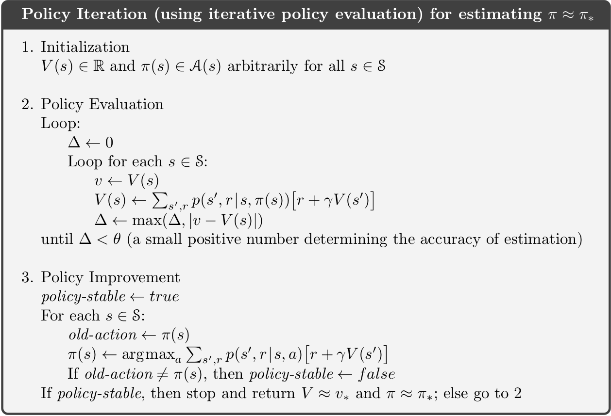
Given the policy improvement theorem we can now improve policies iteratively until we find an optimal policy:
- Pick an arbitrary initial policy \(\pi\).
- Given a policy \(\pi\), estimate \(v_\pi(s)\) via the policy evaluation algorithm.
- Generate a new, improved policy \(\pi' \geq \pi\) by greedily picking \(\pi' = \text{greedy}(v_\pi)\) using Eq. Equation 8.3. If \(\pi'=\pi\) then stop (\(\pi_*\) has been found); otherwise go to Step 2.
The algorithm is given in Fig. 8.2. The sequence of calculations will be: \[\pi_0 \xrightarrow[]{E} v_{\pi_0} \xrightarrow[]{I} \pi_1 \xrightarrow[]{E} v_{\pi_1} \xrightarrow[]{I} \pi_2 \xrightarrow[]{E} v_{\pi_2} \ldots \xrightarrow[]{I} \pi_* \xrightarrow[]{E} v_{*}\] The number of steps of policy iteration needed to find the optimal policy are often low.
8.6 Value Iteration
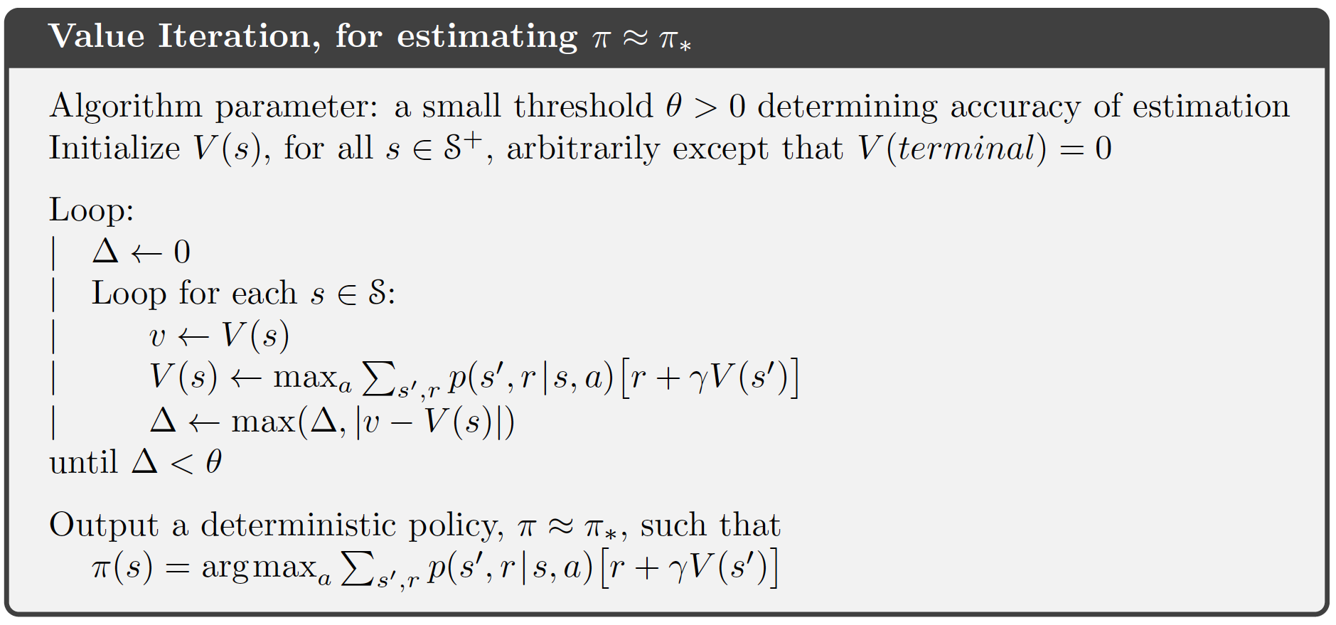
Policy iteration requires full policy evaluation at each iteration step. This could be an computationally expensive process which requires may sweeps of the state space. In value iteration, the policy evaluation is stopped after one sweep of the state space. Value iteration is achieved by turning the Bellman optimality equation into an update rule: \[ v_{k+1}(s) = \max_a \left(r(s,a) + \gamma\sum_{s'} p(s'|s, a)v_k(s')\right) \] Value iteration effectively combines, in each of its sweeps, one sweep of policy evaluation and one sweep of policy improvement, since it performs a greedy update while also evaluating the current policy. Also, it is important to understand that the value-iteration algorithm does not require a policy to work. No actions have to be chosen. Rather, the state-values are updated and after the last step of value-iteration the optimal policy \(\pi_*\) is found:
\[ \pi_*(s) = \arg\max_{a \in \mathcal{A}} \left(r(s,a) + \gamma\sum_{s' \in \mathcal{S}} p(s' | s, a) v_*(s')\right), \] The algorithm is given in Fig. 8.3. Since we do not want an infinite number of iterations we introduce a threshold \(\theta\). The sequence of calculations will be (where G denotes greedy action selection): \[v_{0} \xrightarrow[]{EI} v_{1} \xrightarrow[]{EI} v_{2} \ldots \xrightarrow[]{EI} v_{*} \xrightarrow[]{G} \pi_{*}\]
8.7 Generalized policy iteration
Generalised Policy Iteration (GPI) is the process of letting policy evaluation and policy improvement interact, independent of granularity. For instance, improvement/evaluation can be performed by doing complete sweeps of the state space (policy iteration), or improve the state-value using a single sweep of the state space (value iteration). GPI can also do asynchronous updates of the state-value where states are updated individually, in any order. This can significantly improve computation. Examples on asynchronous DP are
In-place DP mentioned in Section Module 8.3 where instead of keeping a copy of the old and new value function in each value-iteration update, you can just update the value functions in-place. Hence asynchronous updates in other parts of the state-space will directly be affected resulting in faster updates.
Prioritized sweeping where we keep track of how “effective” or “significant” updates to our state-values are. States where the updates are more significant are likely further away from converging to the optimal value. As such, we would like to update them first. For this, we would compute the Bellman error: \[|v_{k+1}(s) - v_k(s)|,\] and keep these values in a priority queue. You can then efficiently pop the top of it to always get the state you should update next.
Prioritize local updates where you update nearby states given the current state, e.g. if your robot is in a particular region of the grid, it is much more important to update nearby states than faraway ones.
GPI works and will convergence to the optimal policy and optimal value function if the states are visited (in theory) an infinite number of times. That is, you must explore the whole state space for GPI to work.
8.8 Example - Factory Storage
Let us consider Exercise 6.6.4 where a factory has a storage tank with a capacity of 4 \(\mathrm{m}^{3}\) for temporarily storing waste produced by the factory.
NoteColab - Before the lecture
8.9 Summary
Read Chapter 4.8 in Sutton and Barto (2018).
8.10 Exercises
Below you will find a set of exercises. Always have a look at the exercises before you meet in your study group and try to solve them yourself. Are you stuck, see the help page. Sometimes hints and solutions can be revealed. Beware, you will not learn by giving up too early. Put some effort into finding a solution!
8.10.1 Exercise - Gambler’s problem
We work with the gambler’s problem you modelled as an MDP in Exercise 6.6.3.
Consider this section in the Colab notebook to see the questions. Use your own copy if you already have one.
8.10.2 Exercise - Maintenance problem
At the beginning of each day a piece of equipment is inspected to reveal its actual working condition. The equipment will be found in one of the working conditions \(s = 1,\ldots, N\) where the working condition \(s\) is better than the working condition \(s+1\).
The equipment deteriorates in time. If the present working condition is \(s\) and no repair is done, then at the beginning of the next day the equipment has working condition \(s'\) with probability \(q_{ss'}\). It is assumed that \(q_{ss'}=0\) for \(s'<s\) and \(\sum_{s'\geq s}q_{ss'}=1\).
The working condition \(s=N\) represents a malfunction that requires an enforced repair taking two days. For the intermediate states \(s\) with \(1<s<N\) there is a choice between preventively repairing the equipment and letting the equipment operate for the present day. A preventive repair takes only one day. A repaired system has the working condition \(s=1\).
The cost of an enforced repair upon failure is \(C_{f}\) and the cost of a preemptive repair in working condition \(s\) is \(C_{p,s}\). We wish to determine a maintenance rule which minimizes the repair cost.
The problem can be formulated as an MDP. Since an enforced repair takes two days and the state of the system has to be defined at the beginning of each day, we need an auxiliary state for the situation in which an enforced repair is in progress already for one day.
Consider this section in the Colab notebook to see the questions. Use your own copy if you already have one.
8.10.3 Exercise - Car rental
Consider the car rental problem in Exercise 7.8.2. Note the inventory dynamics (number of cars) at each parking lot is independent of the other given an action \(a\). Let us consider Location 1 and assume that we are in state \(x\) and chose action \(a\).
The reward equals the reward of rentals minus the cost of movements. Note we have \(\bar{x} = x - a\) and \(\bar{y} = x + a\) after movement. Hence \[r(s,a) = \mathbb{E}[10(\min(D_1, \bar{x}) + \min(D_2, \bar{y}) )-2\mid a \mid]\] where \[\mathbb{E}[\min(D, z)] = \sum_{i=0}^{z-1} i\Pr(D = i) + \Pr(D \geq z)z.\]
Let us have a look at the state transition, the number of cars after rental requests \(\bar{x} - \min(D_1, \bar{x})\). Next, the number of returned cars are added: \(\bar{x} - \min(D_1, \bar{x}) + H_1\). Finally, note that if this number is above 20 (parking lot capacity), then we only have 20 cars, i.e. the inventory dynamics (number of cars at the end of the day) is \[X = \min(20, \bar{x} - \min(D_1, \bar{x}) + H_1))).\] Similar for Location 2, if \(\bar{y}= y+a\) we have \[Y = \min(20, \bar{y} - \min(D_2, \bar{y}) + H_2)).\]
Since the dynamics is independent given action a, the transition probabilities can be split: \[ p((x',y') | (x,y), a) = p(x' | x, a) p(y' | y, a).\]
Let us consider Location 1. If \(x' < 20\) then \[ \begin{align} p(x' | x, a) &= \Pr(x' = x-a - \min(D_1, x-a) + H_1)\\ &= \Pr(x' = \bar{x} - \min(D_1, \bar{x}) + H_1)\\ &= \Pr(H_1 - \min(D_1, \bar{x}) = x' - \bar{x}) \\ &= \sum_{i=0}^{\bar{x}} \Pr(\min(D_1, \bar{x}) = i)\Pr(H_1 = x' - \bar{x} + i) \\ &= \sum_{i=0}^{\bar{x}}\left( (\mathbf{1}_{(i<\bar{x})} \Pr(D_1 = i) + \mathbf{1}_{(i=\bar{x})} \Pr(D_1 \geq \bar{x}))\Pr(H_1 = x' - \bar{x} + i)\right) \\ &= p(x' | \bar{x}). \end{align} \]
If \(x' = 20\) then \[ \begin{align} p(x' | x, a) &= \Pr(20 \leq \bar{x} - \min(D_1, \bar{x}) + H_1)\\ &= \Pr(H_1 - \min(D_1, \bar{x}) \geq 20 - \bar{x}) \\ &= \sum_{i=0}^{\bar{x}} \Pr(\min(D_1, \bar{x}) = i)\Pr(H_1 \geq 20 - \bar{x} + i) \\ &= \sum_{i=0}^{\bar{x}}\left( (\mathbf{1}_{(i<\bar{x})} \Pr(D_1 =i) + \mathbf{1}_{(i=\bar{x})} \Pr(D_1 \geq \bar{x}))\Pr(H_1 \geq 20 - \bar{x} + i)\right)\\ &= p(x' = 20 | \bar{x}). \end{align} \]
Similar for Location 2. That is we need to calculate and store \(p(x'| \bar{x})\) and \(p(y'| \bar{y})\) to find \[ p((x',y') | (x,y), a) = p(x' | \bar{x} = x-a) p(y' | \bar{y} = y+a).\]
Consider this section in the Colab notebook to see the questions. Use your own copy if you already have one.