Module 11 Introduction to tidyverse and RMarkdown
The tidyverse is a collection of R packages designed for data science. RMarkdown documents support the concept of literate programming where you weave R code together with text (written in Markdown) to produce elegantly formatted documents.
A template project for this module is given on Posit Cloud (open it and use it while reading the notes).
Learning path diagram
11.1 Learning outcomes
By the end of this module, you are expected to be able to:
- Describe what the tidyverse package is.
- Explain the ideas behind reproducible reports and literal programming.
- Create your first RMarkdown document and add some code and text.
The learning outcomes relate to the overall learning goals number 7, 17 and 18 of the course.
11.2 The tidyverse package
The tidyverse is a collection of R packages designed for data science. All packages share an underlying design philosophy, grammar, and data structures.
The core tidyverse includes the packages that you are likely to use in everyday data analyses. In tidyverse 1.3.0, the following packages are included in the core tidyverse:
dplyr provides a grammar of data manipulation, providing a consistent set of verbs that solve the most common data manipulation challenges. We are going to use dplyr in Module 13.
ggplot2 is a system for declaratively creating graphics, based on The Grammar of Graphics. You provide the data, tell ggplot2 how to map variables to aesthetics, what graphical primitives to use, and it takes care of the details. We are going to use ggplot in Module 14.
tidyr provides a set of functions that help you get to tidy data. Tidy data is data with a consistent form: in brief, every variable goes in a column, and every column is a variable.
readr provides a fast and friendly way to read rectangular data (like csv, tsv, and fwf). It is designed to flexibly parse many types of data found in the wild, while still cleanly failing when data unexpectedly changes. We are going to use dplyr in Module 12.
purrr enhances R’s functional programming (FP) toolkit by providing a complete and consistent set of tools for working with functions and vectors. Once you master the basic concepts, purrr allows you to replace many for loops with code that is easier to write and more expressive. This package is not covered in this course.
tibble is a modern re-imagining of the data frame, keeping what time has proven to be effective, and throwing out what has not. Tibbles are data frames that are lazy and surly: they do less and complain more forcing you to confront problems earlier, typically leading to cleaner, more expressive code. We are going to use tibbles in Module 13.
stringr provides a cohesive set of functions designed to make working with strings as easy as possible. You have already worked a bit with stringr in Exercise 8.7.8
forcats provides a suite of useful tools that solve common problems with factors. R uses factors to handle categorical variables, variables that have a fixed and known set of possible values. This package is not covered in this course.
Small introductions (with examples) to the packages are given on their documentation pages (follow the links above). The tidyverse also includes many other packages with more specialized usage. They are not loaded automatically with library(tidyverse), so you will need to load each one with its own call to library().
11.3 Writing reproducible reports
The concept of literate programming was originally introduced by Donald Knuth in 1984. In a nutshell, Knuth envisioned a new programming paradigm where computer scientists focus on weaving code together with text as documentation.
That is, when we do an Analytics project, we are interested in writing reports containing both R code for importing data, wrangling and analysis. Moreover, at the same time, the document should contain our comments about the code, plots, analysis, results, etc. The document is then rendered to an output format such as html, pdf or Word which is presented to the decision maker. Note the document can be seen as the “the source code” for the report communicated to the decision maker.
Some developers have created tools to enable others to write better literate programs. They use a markup language made for authoring. We are going to focus on RMarkdown. In RMarkdown documents you can weave R code together with text (written in Markdown) to produce elegantly formatted output.
In fact this book is written in RMarkdown by using
- a set of RMarkdown documents bound together as a collection using the bookdown package,
- rendered to a web page using RStudio,
- shared on GitHub,
- built by GitHub Actions,
- and published on GitHub Pages.
This may seem complicated at first. However, after setup, it makes life much easier, since we can
- update the book easier,
- share and collaborate on the book easier,
- update the web page automatically,
- keep history of the book source,
- keep the book source at a single location.
RMarkdown documents are reproducible. Anybody who works with data has at some point heard a colleague say ‘Well, it works on my computer’, expressing dismay at the fact that you cannot reproduce their results. Ultimately, reproducible means that the results can be reproduced given access to the original data, software, and code. In practice it may be hard to make your project totally reproducible. For instance, people may be using a different operating system, other versions of the software, etc. That is, there are different levels of reproducibility. In this course, we will focus on RMarkdown only. See Module 11 for more info about levels of reproducibility.
An introduction to RMarkdown is given in Chapters 3 and 4 of the DataCamp course Communicating with Data in the Tidyverse. Note that you may skip Chapters 1 and 2 and still understand most of the questions in Chapters 3 and 4 (otherwise just see the solution). You are expected to have completed the chapters before continuing this module!
The RMarkdown cheatsheet may be useful. Find the newest version in RStudio Help > Cheatsheets. All chunk options for R code can be seen here.
11.4 Tibbles
Tibbles are a modern data frame, keeping what time has proven to be effective, and throwing out what is not. Tibbles are more strict compared to data frames e.g. they do not change variable names or types, do not do partial matching and complain more e.g. when a variable does not exist. This forces you to confront problems earlier, typically leading to cleaner, more expressive code. Moreover, tibbles have an enhanced print method and can have columns that are lists.
Let us see a few examples:
tbl1 <- tibble(name = c("Lars", "Susan", "Hans"), age = c(23, 56, 45))
tbl1
#> # A tibble: 3 × 2
#>   name    age
#>   <chr> <dbl>
#> 1 Lars     23
#> 2 Susan    56
#> 3 Hans     45
tbl2 <- tibble(x = 1:3, y = list(1:5, 1:10, 1:20))
tbl2
#> # A tibble: 3 × 2
#>       x y
#>   <int> <list>
#> 1     1 <int [5]>
#> 2     2 <int [10]>
#> 3     3 <int [20]>
tbl3 <- as_tibble(mtcars)
tbl3
#> # A tibble: 32 × 11
#>      mpg   cyl  disp    hp  drat    wt  qsec    vs    am  gear  carb
#>    <dbl> <dbl> <dbl> <dbl> <dbl> <dbl> <dbl> <dbl> <dbl> <dbl> <dbl>
#>  1  21       6  160    110  3.9   2.62  16.5     0     1     4     4
#>  2  21       6  160    110  3.9   2.88  17.0     0     1     4     4
#>  3  22.8     4  108     93  3.85  2.32  18.6     1     1     4     1
#>  4  21.4     6  258    110  3.08  3.22  19.4     1     0     3     1
#>  5  18.7     8  360    175  3.15  3.44  17.0     0     0     3     2
#>  6  18.1     6  225    105  2.76  3.46  20.2     1     0     3     1
#>  7  14.3     8  360    245  3.21  3.57  15.8     0     0     3     4
#>  8  24.4     4  147.    62  3.69  3.19  20       1     0     4     2
#>  9  22.8     4  141.    95  3.92  3.15  22.9     1     0     4     2
#> 10  19.2     6  168.   123  3.92  3.44  18.3     1     0     4     4
#> # ℹ 22 more rows
tbl4 <- tribble(
  ~x, ~y, ~z,
  #--|--|----
  "a", 2, 3.6,
  "b", 1, 8.5
)
tbl4
#> # A tibble: 2 × 3
#>   x         y     z
#>   <chr> <dbl> <dbl>
#> 1 a         2   3.6
#> 2 b         1   8.5
Note that we can always coerce a data frame to a tibble (tbl3) or create it directly using tibble. Another way to create a tibble is with tribble. Here column headings are defined by formulas (i.e. they start with ~), and entries are separated by commas. This makes it possible to lay out small amounts of data in easy to read form.
Tibbles have a refined print method that shows only the first 10 rows along with the number of columns that will fit on your screen. This makes it much easier to work with large data. In addition to its name, each column reports its type. Hence, your console is not overwhelmed with data. To see a full view of the data, you can use RStudio’s built-in data viewer:
11.5 Recap
tidyverse is a collection of R packages designed for data science. All packages share an underlying design philosophy, grammar, and data structures.
RMarkdown is an example of literate programming.
The core tidyverse includes the packages that you are likely to use in everyday data analyses.
The concept of literate programming is a programming paradigm which focuses on weaving code together with text as documentation. That is, we are interested in writing reports containing both text and R code for importing data, wrangling and analysis.
Reproducibility means that the results can be reproduced given access to the original data, software, and code.
In practice it may be hard to make your project totally reproducible. That is, there are different levels of reproducibility.
RMarkdown documents are an attempt to make reproducible documents and combine R code and markdown text.
All chunk options for R code in RMarkdown documents can be seen here.
The RMarkdown cheatsheet may be useful. Find the newest version in RStudio Help > Cheatsheets. For Markdown syntax see Help > Markdown Quick Reference.
Tibbles are a modern data frame, keeping what time has proven to be effective, and throwing out what is not.
Tibbles are more strict compared to data frames e.g. they do not change variable names or types, do not do partial matching and complain more e.g. when a variable does not exist.
Tibbles have an enhanced
printmethod and can have columns that are lists.
11.6 Exercises
Below you will find a set of exercises. Always have a look at the exercises before you meet in your study group and try to solve them yourself. Are you stuck, see the help page. Some of the solutions to each exercise can be seen by pressing the button at each question. Beware, you will not learn by giving up too early. Put some effort into finding a solution! Always practice using shortcuts in RStudio (see Tools > Keyboard Shortcuts Help).
Go to the Tools for Analytics workspace and download/export the TM11 project. Open it on your laptop and have a look at the files in the exercises folder which can be used as a starting point.
11.6.1 Exercise (your first RMarkdown exercise)
Load the tfa package:
# If tfa package is not installed then run
# install.packages("remotes")
# remotes::install_github("bss-osca/tfa-package", upgrade = FALSE)
library(tfa)
The package contains templates for exercises etc. Go to File > New File > R Markdown…. In the pop-up box select From template in the left column and then TFA Exercise. Press Ok and a new RMarkdown document will be opened.
Change the meta text (e.g. the title and add your name) in the yaml.
Render/compile the document by pressing the Knit button (or Ctrl+Shift+K).
- Change
echo = TRUEtoecho = FALSEin the first chunksetupand render the document. What has happened?
You can easily go to a chunk using the navigation in the bottom left of the source window.
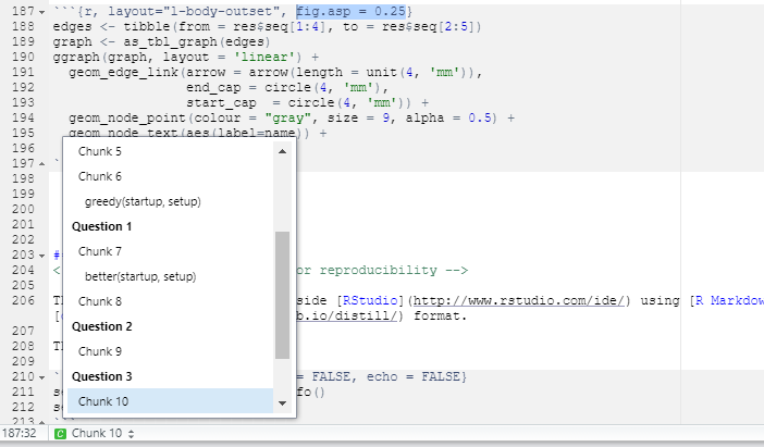
Try to change
fig.asp = 0.25to e.g. 0.5 in Chunk 10 (and seteval = TRUE). What happens? Note: You may need to callinstall.packages("ggraph")if getError in library(ggraph) : there is no package called 'ggraph'.Create a new section
## Question 4and add text in italic: What is the sum of all setup costs?
- Add a code chunk solving Question 4 above.
- Add a line of text with the result.