Module 8 R basics and workflows

This module contains an introduction to using R, the syntax, data types etc. Coding in R is, as VBA, best learnt by trying it out and learn by trial and error. Hence the modules often contains links to interactive tutorials.

A template project for this module is given on Posit Cloud (open it and use it while reading the notes).

Learning path diagram

It is recommended that you follow the green learning path; however, you may like a different learning style. In the learning path diagram, there are links to alternative online content (video or reading). Note this is an alternative to the standard learning path that you may use instead (you should not do both). The learning path may also have extra content, that is NOT a part of syllabus (only look at it if you want more info)!

8.1 Learning outcomes

By the end of this module, you are expected to have:

• Tried R and RStudio.
• Learned how the RStudio IDE works.
• Finished your first course on DataCamp.
• Solved your first exercises.

The learning outcomes relate to the overall learning goals number 2, 5, 6, 8, 11, 13 and 15 of the course.

8.2 Working with R at the command line in RStudio

R is a programming language and free software environment. The R language is widely used among statisticians and data miners for data analysis. To run R you need to install it on your laptop or use a cloud version. We will use R via RStudio. First time users often confuse the two. At its simplest, R is like a car’s engine while RStudio is like a car’s dashboard as illustrated in Figure 8.1.

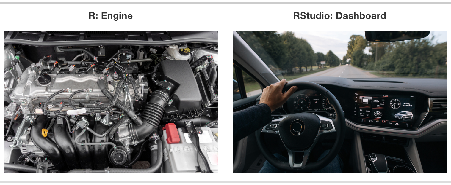
Figure 8.1: Analogy of difference between R and RStudio.

More precisely, R is a programming language that runs computations, while RStudio is an integrated development environment (IDE) that provides an interface by adding many convenient features and tools. So just as the way of having access to a speedometer, rearview mirrors, and a navigation system makes driving much easier, using RStudio’s interface makes using R much easier as well. RStudio can be accessed using both your laptop version or Posit Cloud. We will assume that you are using R via Posit Cloud if not stated otherwise.

Compared to Excel, the benefit of using Excel is that the initial learning curve is quite minimal, and most analysis can be done via point-and-click on the top panel. Once a user imports their data into the program, it’s not exceedingly hard to make basic graphs and charts. R is a programming language, however, meaning the initial learning curve is steeper. It will take you some time to become familiar with the interface and master the various functions. Luckily, using R can quickly become second-nature with practice. For a detailed comparison you may see Excel vs R: A Brief Introduction to R by Jesse Sadler.

Compared to VBA, R is an interpreted language; users typically access it through a command-line or script file. To run VBA you need to compile and execute it.

Launch Posit Cloud (follow this link to get to the correct project). An personal copy of the project is now created for you. Consider the panes:

• Console (left)
• Environment/History (tabbed in upper right)
• Files/Plots/Packages/Help (tabbed in lower right)

FYI: you can change the default location of the panes, among many other things: Customizing RStudio.

Now that you are set up with R and RStudio, you are probably asking yourself, “OK - now how do I use R?”. The first thing to note is that unlike other software programs like Excel or SPSS that provide point-and-click interfaces, R is an interpreted language. This means you have to type in commands written in R code. In other words, you have to code/program in R. Note that we will use the terms “coding” and “programming” interchangeably.

Go into the Console, where we interact with the live R process.

Make an assignment and then inspect the object you just created:

x <- 3 * 4
x
#> [1] 12

All R statements where you create objects – “assignments” – have this form:

object_name <- value

and in my head I hear, e.g., “x equals 12”. You will make lots of assignments and the operator <- is a pain to type. Do not be lazy and use =, although it would work, because it will just sow confusion later. Instead, utilize RStudio’s keyboard shortcut: Alt+- (the minus sign).

Note that RStudio automatically surrounds <- with spaces, which demonstrates a useful code formatting practice. Give your eyes a break and use spaces.

RStudio offers many handy keyboard shortcuts. Also, check Tools > Keyboard Shortcuts Help which brings up a keyboard shortcut reference card.

Object names cannot start with a digit and cannot contain certain other characters such as a comma or a space. You are advised to adopt a coding convention; some use snake case others use camel case. Choose the naming convention you like best in your study group. But stick only to one of them.

this_is_snake_case   # note you do not use capital letters here
thisIsCamelCase      # you start each word with a capital letter

Make another assignment:

this_is_a_long_name <- 2.5

To inspect this, try out RStudio’s completion facility: type the first few characters, press TAB, add characters until you agree, then press return.

In VBA you have procedures and functions. In R we only use functions which always return an object. R has a mind-blowing collection of built-in functions that are accessed like so:

function_name(arg1 = val1, arg2 = val2, ...)

Let’s try function seq() which makes regular sequences of numbers and at the same time demo more helpful features of RStudio.

Type se and hit TAB. A pop-up shows you possible completions. Specify seq() by typing more or use the up/down arrows to select. Note the floating tool-tip-type help that pops up, reminding you of a function’s arguments. If you want even more help, press F1 as directed to get the full documentation in the help tab of the lower right pane. Now open the parentheses and note the automatic addition of the closing parenthesis and the placement of the cursor in the middle. Type the arguments 1, 10 and hit return.

seq(1, 10)
#>  [1]  1  2  3  4  5  6  7  8  9 10

The above also demonstrates something about how R resolves function arguments. Type seq and press F1 or type:

?seq

The Help tab of the lower right pane will show the help documentation of function seq with a description of usage, arguments, return value etc. Note all function arguments have names. You can always specify arguments using name = value form. But if you do not, R attempts to resolve by position. So above, it is assumed that we want a sequence from = 1 that goes to = 10. Since we did not specify step size, the default value of by in the function definition is used, which ends up being 1 in this case. Note since the default value for from is 1, the same result is obtained by typing:

seq(to = 10)
#>  [1]  1  2  3  4  5  6  7  8  9 10

Make this assignment and note similar help with quotation marks.

yo <- "hello world"

If you just create an assignment, you do not see the value. You may see the value by:

yo          # same as print(yo)
#> [1] "hello world"
print(yo)  
#> [1] "hello world"

Now look at your Environment tab in the upper right pane where user-defined objects accumulate. You can also get a listing of these objects with commands:

objects()
#>  [1] "add_graph_legend"     "addIconOld"           "addIconTasks"         "addSolution"         
#>  [5] "create_learning_path" "ctrSol"               "dat"                  "eval_inline"         
#>  [9] "exercises_r_text"     "g"                    "learning_path_text_r" "link_excel_file"     
#> [13] "link_excel_file_text" "link_rcloud_text"     "link_slide_file_text" "module_name"         
#> [17] "module_number"        "module_number_prefix" "project_name_prefix"  "sheet_name_prefix"   
#> [21] "strExercises"         "strLPath"             "this_is_a_long_name"  "x"                   
#> [25] "yo"
ls()
#>  [1] "add_graph_legend"     "addIconOld"           "addIconTasks"         "addSolution"         
#>  [5] "create_learning_path" "ctrSol"               "dat"                  "eval_inline"         
#>  [9] "exercises_r_text"     "g"                    "learning_path_text_r" "link_excel_file"     
#> [13] "link_excel_file_text" "link_rcloud_text"     "link_slide_file_text" "module_name"         
#> [17] "module_number"        "module_number_prefix" "project_name_prefix"  "sheet_name_prefix"   
#> [21] "strExercises"         "strLPath"             "this_is_a_long_name"  "x"                   
#> [25] "yo"

If you want to remove the object named yo, you can do this:

rm(yo)

To remove everything:

rm(list = ls())

or click the broom in RStudio’s Environment pane.

8.3 Your first DataCamp course

DataCamp is an online platform for learning data science. We are going to use the platform for online tutorials. First, sign up to the organization Tools for analytics at DataCamp using your university e-mail here (IMPORTANT do this before running the course/tutorial below!).

DataCamp runs all the courses in your browser. That is, R is run on a server and you do not use RStudio here. The first course gives an Introduction to R. You are expected to have completed the course before continuing this module!

8.4 Pipes

Most functions support the pipe operator which is a powerful tool for clearly expressing a sequence of multiple operations. The native pipe operator is |>, but you may also use the pipe operator %>%, that comes from the magrittr package and is loaded automatically when you load tidyverse.

To insert the pipe operator, you may use the RStudio keyboard shortcut Ctrl+Shift+M. This by default uses the %>% pipe operator. If you want to use the native open Tools > Global Options… > Code and check mark Use native pipe operator … (recommended).

Consider the following code:

# calculate x as a sequence of operations
x <- 16
x <- sqrt(x)
x <- log2(x)
x
#> [1] 2
# same as
y <- log2(sqrt(16))
y
#> [1] 2

Note we here calculate x using a sequence of operations:

\[ \mbox{original data (x)} \rightarrow \mbox{ sqrt } \rightarrow \mbox{ log2 }. \]

That is, we take what is left of the arrow (the object x) and put it into the function on the right of the arrow. These operations can be done using the pipe operator:

library(tidyverse)
x <- 16
x <- x |>
   sqrt() |>
   log2()
x
#> [1] 2

In general, the pipe sends the result of the left side of the pipe to be the first argument of the function on the right side of the pipe. That is, you may have other arguments in your functions:

16 |> sqrt() |> log2()
#> [1] 2
16 |> sqrt() |> log(base = 2)   # equivalent
#> [1] 2

The above example is simple but illustrates that you can use pipes to skip intermediate assignment operations. Later you will do more complex pipes when we consider data wrangling. For instance,

mtcars |> select(cyl, gear, hp, mpg) |> filter(gear == 4, cyl == 4)
#>                cyl gear  hp  mpg
#> Datsun 710       4    4  93 22.8
#> Merc 240D        4    4  62 24.4
#> Merc 230         4    4  95 22.8
#> Fiat 128         4    4  66 32.4
#> Honda Civic      4    4  52 30.4
#> Toyota Corolla   4    4  65 33.9
#> Fiat X1-9        4    4  66 27.3
#> Volvo 142E       4    4 109 21.4

selects the columns related to cylinders, gears, horse power and miles, and then rows with cars having four cylinders and gears. For a more detailed introduction to pipes see Chapter 18 in H. Wickham (2017).

8.5 RStudio projects

One day you will need to quit R, do something else and return to your analysis later.

One day you will have multiple analyses going that use R and you want to keep them separate.

One day you will need to bring data from the outside world into R and send numerical results and figures from R back out into the world.

To handle these real life situations, you need to store your work in a project that keeps all the files associated with a project organized together (such as input data, R scripts, analytical results and figures). RStudio has built-in support for this via its [projects][rstudio-using-projects]. You may think of a project as a folder where you store all you work.

On Posit Cloud you create a project inside a workspace. Projects have already been made for most modules. However, let us try to create a project in your Your Workspace workspace. Expand the left menu and select your Your Workspace workspace. Press the New Project button and select New RStudio Project. The project is now created and you can rename it in the upper left corner. Go back to the project 01-module-12 in the Tools for Analytics workspace that we will use for the remaining of the module.

For RStudio on your laptop you create a project for the rest of this module by doing this: File > New Project… > New Directory > New Project >. The directory name you choose here will be the project name. Call it whatever you want (or follow me for convenience). I used tfa_testing in my tmp directory (that is tfa_testing is now a subfolder of tmp.

You now need a way to store R code in your project. We will use 2 ways of storing your code. An R script file or an R Markdown document. Normally you store lines of R code in a script file that you need to run.

R Markdown provides an easy way to produce a rich, fully-documented reproducible analysis. Here you combine text, figures and metadata needed to reproduce the analysis from the beginning to the end in a single file. R Markdown compiles to nicely formatted HTML, PDF, or Word. We are going to use R Markdown for larger projects (e.g. the mandatory R report). We will come back to R Markdown later.

8.5.1 Storing your code in a script file

R code can be stored in a script file with file suffix .R. A script file contains a line for each R command to run (think of each line as a command added to the console). Create a new script file File > New File > R Script. Let us add some R code to the file:

# this is a comment
a <- 2
b <- -3
sig_sq <- 0.5
x <- runif(40)
y <- a + b * x + rnorm(40, sd = sqrt(sig_sq))
(avg_x <- mean(x))
write(avg_x, "avg_x.txt")
plot(x, y)
abline(a, b, col = "purple")
dev.print(pdf, "toy_line_plot.pdf")

Save the file as testing.R Now run each line by setting the cursor at the first line, hit Ctrl+Enter (runs the line in the Console and moves the cursor to the next line). Repeat Ctrl+Enter until you have run all the lines. Alternatively you may select all the code and hit Ctrl+Enter.

Change some things in your code. For instance set a sample size n at the top, e.g. n <- 40, and then replace all the hard-wired 40’s with n. Change some other minor, but detectable, stuff, e.g. alter the sample size n, the slope of the line b, the color of the line etc. Practice the different ways to rerun the code:

• Walk through line by line by keyboard shortcut (Ctrl+Enter) or mouse (click “Run” in the upper right corner of editor pane).

• Source the entire document by entering source('testing.R') in the Console or use keyboard shortcut (Shift+Ctrl+S) or mouse (click “Source” in the upper right corner of editor pane or select from the mini-menu accessible from the associated down triangle).

• Source with echo from the Source mini-menu.

Try to get an overview of the different planes and tabs. For instance in the Files tab (lower right plane) you can get an overview of your project files. You may also see this video about projects.

8.6 Recap

R is a programming language that runs computations, while RStudio is an integrated development environment (IDE) that provides an interface by adding many convenient features and tools.

Adopt a naming convention. Either use snake case or use camel case. Choose the naming convention you like best in your study group. But stick only to one of them.

Store your work in a project that keeps all the files associated with a project organized together (such as input data, R scripts, analytical results and figures). You may think of a project as a folder where you store all your work.

This workflow will serve you well in the future:

• Create an RStudio project for an analytical project (a project for most modules is already created in Posit Cloud)
• Keep inputs there (we will soon talk about importing)
• Keep scripts there; edit them, run them in bits or as a whole from there
• Keep outputs there (like the PDF written above)

Avoid using the mouse for pieces of your analytical workflow, such as loading a dataset or saving a figure. This is extremely important for the reproducibility and for making it possible to retrospectively determine how a numerical table or PDF was actually produced.

Learn and use shortcuts as much as possible. For instance Alt+- for the assignment operator and Ctrl+Shift+M for the pipe operator. A reference card of shortcuts can be seen using Alt+Shift+K.

Store your R commands in a script file and R scripts with a .R suffix.

Comments start with one or more # symbols. Use them. RStudio helps you (de)comment selected lines with Ctrl+Shift+C (Windows and Linux) or Cmd+Shift+C (Mac).

Values saved in R are stored in Objects.

The interactive DataCamp course gave an introduction to some basic programming concepts and terminology:

• Data types: integers, doubles/numerics, logicals, and characters. Integers are values like -1, 0, 2, 4092. Doubles or numerics are a larger set of values containing both the integers but also fractions and decimal values like -24.932 and 0.8. Logicals are either TRUE or FALSE while characters are text such as “Hamilton”, “The Wire is the greatest TV show ever”, and “This ramen is delicious.” Note that characters are often denoted with the quotation marks around them.

• Vectors: a series of values. These are created using the c() function, where c() stands for “combine” or “concatenate.” For example, c(6, 11, 13, 31, 90, 92) creates a six element series of positive integer values .

• Factors: categorical data are commonly represented in R as factors. Categorical data can also be represented as strings.

• Data frames: rectangular spreadsheets. They are representations of datasets in R where the rows correspond to observations and the columns correspond to variables that describe the observations.

• Lists are general containers that can be used to store a set of different objects under one name (that is, the name of the list) in an ordered way. These objects can be matrices, vectors, data frames, even other lists, etc. It is not even required that these objects are related to each other in any way.

• Comparison operators known to R are:

  • < for less than,
  • > for greater than,
  • <= for less than or equal to,
  • >= for greater than or equal to,
  • == for equal to each other (and not = which is typically used for assignment!),
  • != not equal to each other.

A pipe (|>) sends the result of the left side of the pipe to be the first argument of the function on the right side of the pipe. Use pipes if you have many intermediate assignment operations.

You may also have a look at the slides for this module .

8.7 Exercises

Below you will find a set of exercises. Always have a look at the exercises before you meet in your study group and try to solve them yourself. Are you stuck, see the help page. Some of the solutions to each exercise can be seen by pressing the button at each question. Beware, you will not learn by giving up too early. Put some effort into finding a solution! Always practice using shortcuts in RStudio (see Tools > Keyboard Shortcuts Help).

Go to the Tools for Analytics workspace and download/export the TM8 project. Open it on your laptop and have a look at the files in the exercises folder which can be used as a starting point.

8.7.1 Exercise (group work)

You are not expected to start solving this exercise before you meet in your group.

You have all been allocated into groups. During the course, you are expected to solve the R exercises in these groups. Before you start, it is a good idea to agree on a set of group rules:

1. It is a good idea to have a shared place for your code. Have a look at the section Working in groups and decide on a place to share your code.
2. Create a shared folder where you can share your projects.
3. Agree on a coding convention.

8.7.2 Exercise (piping)

Solve this exercise using a script file (e.g. exercises/pipe.R which already has been created). Remember that you can run a line in the file using Ctrl+Enter.

The pipe |> can be used to perform operations sequentially without having to define intermediate objects (Ctrl+Shift+M). Have a look at the dataset mtcars:

head(mtcars)
?mtcars

The pipe

library(tidyverse)
mtcars |> select(cyl, gear, hp, mpg) |> filter(gear == 4 & cyl == 4)
#>                cyl gear  hp  mpg
#> Datsun 710       4    4  93 22.8
#> Merc 240D        4    4  62 24.4
#> Merc 230         4    4  95 22.8
#> Fiat 128         4    4  66 32.4
#> Honda Civic      4    4  52 30.4
#> Toyota Corolla   4    4  65 33.9
#> Fiat X1-9        4    4  66 27.3
#> Volvo 142E       4    4 109 21.4

selects the columns related to cylinders, gears, horse power and miles, and then rows with cars having four cylinders and (operator &) gears.

Solution

mtcars |> 
   select(mpg, hp, am, gear)
#>                      mpg  hp am gear
#> Mazda RX4           21.0 110  1    4
#> Mazda RX4 Wag       21.0 110  1    4
#> Datsun 710          22.8  93  1    4
#> Hornet 4 Drive      21.4 110  0    3
#> Hornet Sportabout   18.7 175  0    3
#> Valiant             18.1 105  0    3
#> Duster 360          14.3 245  0    3
#> Merc 240D           24.4  62  0    4
#> Merc 230            22.8  95  0    4
#> Merc 280            19.2 123  0    4
#> Merc 280C           17.8 123  0    4
#> Merc 450SE          16.4 180  0    3
#> Merc 450SL          17.3 180  0    3
#> Merc 450SLC         15.2 180  0    3
#> Cadillac Fleetwood  10.4 205  0    3
#> Lincoln Continental 10.4 215  0    3
#> Chrysler Imperial   14.7 230  0    3
#> Fiat 128            32.4  66  1    4
#> Honda Civic         30.4  52  1    4
#> Toyota Corolla      33.9  65  1    4
#> Toyota Corona       21.5  97  0    3
#> Dodge Challenger    15.5 150  0    3
#> AMC Javelin         15.2 150  0    3
#> Camaro Z28          13.3 245  0    3
#> Pontiac Firebird    19.2 175  0    3
#> Fiat X1-9           27.3  66  1    4
#> Porsche 914-2       26.0  91  1    5
#> Lotus Europa        30.4 113  1    5
#> Ford Pantera L      15.8 264  1    5
#> Ferrari Dino        19.7 175  1    5
#> Maserati Bora       15.0 335  1    5
#> Volvo 142E          21.4 109  1    4

Hint

mtcars |> 
   select(___, ___, ___, ___)

1. Create a pipe that selects columns related to miles, horsepower, transmission and gears.

Solution

mtcars |> 
   select(mpg, hp, am, gear) |> 
   filter(mpg < 20, gear == 4)
#>            mpg  hp am gear
#> Merc 280  19.2 123  0    4
#> Merc 280C 17.8 123  0    4

Hint

mtcars |> 
   select(mpg, hp, am, gear) |> 
   filter(___, ___)

2. Given the answer in 1), filter so cars have miles less than 20 and 4 gears.

Solution

mtcars |> 
   select(mpg, hp, am, gear) |> 
   filter(mpg < 20 | gear == 4)
#>                      mpg  hp am gear
#> Mazda RX4           21.0 110  1    4
#> Mazda RX4 Wag       21.0 110  1    4
#> Datsun 710          22.8  93  1    4
#> Hornet Sportabout   18.7 175  0    3
#> Valiant             18.1 105  0    3
#> Duster 360          14.3 245  0    3
#> Merc 240D           24.4  62  0    4
#> Merc 230            22.8  95  0    4
#> Merc 280            19.2 123  0    4
#> Merc 280C           17.8 123  0    4
#> Merc 450SE          16.4 180  0    3
#> Merc 450SL          17.3 180  0    3
#> Merc 450SLC         15.2 180  0    3
#> Cadillac Fleetwood  10.4 205  0    3
#> Lincoln Continental 10.4 215  0    3
#> Chrysler Imperial   14.7 230  0    3
#> Fiat 128            32.4  66  1    4
#> Honda Civic         30.4  52  1    4
#> Toyota Corolla      33.9  65  1    4
#> Dodge Challenger    15.5 150  0    3
#> AMC Javelin         15.2 150  0    3
#> Camaro Z28          13.3 245  0    3
#> Pontiac Firebird    19.2 175  0    3
#> Fiat X1-9           27.3  66  1    4
#> Ford Pantera L      15.8 264  1    5
#> Ferrari Dino        19.7 175  1    5
#> Maserati Bora       15.0 335  1    5
#> Volvo 142E          21.4 109  1    4

Hint

mtcars |> 
   select(mpg, hp, am, gear) |> 
   filter(___ | ___)

3. Given the answer in 1), filter so cars have miles less than 20 or 4 gears. The “or” operator in R is |.

Solution

mtcars |> 
   filter(mpg < 20, gear == 4) |> 
   select(wt, vs) 
#>             wt vs
#> Merc 280  3.44  1
#> Merc 280C 3.44  1

Hint

mtcars |> 
   filter(mpg < 20, gear == 4) |> 
   select(___, ___) 

4. Create a pipe that filters the cars having miles less than 20 and 4 gears and selects columns related to weight and engine.

Solution

dat <- mtcars 
dat <- filter(dat, mpg < 20, gear == 4) 
dat <- select(dat, wt, vs) 
dat
#>             wt vs
#> Merc 280  3.44  1
#> Merc 280C 3.44  1

Hint

dat <- mtcars 
dat <- filter(dat, ___) 
dat <- select(dat, ___) 
dat

5. Solve Question 4 without the pipe operator.

8.7.3 Exercise (working dir)

Do this exercise from the Console in RStudio.

When reading and writing to local files, your working directory becomes important. You can get and set the working directory using functions getwd and setwd.

Set the working directory to the project directory using the menu: Session > Set Working Directory > To Project Directory. Now let us create some files:

   library(tidyverse)
   dir.create("subfolder", showWarnings = FALSE) 
   write_file("Some text in a file", file = "test1.txt")
   write_file("Some other text in a file", file = "subfolder/test2.txt")

1. Which folders and files have been created? You may have a look in the Files tab in RStudio.

We can read the file again using:

read_file("test1.txt")

Solution

read_file("subfolder/test2.txt")

Hint

read_file("subfolder/___")

2. Read the file test2.txt.

3. Set the working directory to subfolder using function setwd. Note that setwd supports relative paths. Check that you are in the right working directory using getwd. You may also have a look at the files in the directory using function list.files.

Solution

setwd("subfolder")  # done in Q3
read_file("../test1.txt")
read_file("test2.txt")

Hint

setwd("subfolder")  # done in Q3
read_file("../___")
read_file("___")

4. Read files test1.txt and test2.txt. Note that in relative paths ../ means going to the parent folder. What is different compared to Question 2?

8.7.4 Exercise (vectors)

Solve this exercise using a script file.

Solution

n <- 100
n * (n+1) / 2
#> [1] 5050

1. What is the sum of the first 100 positive integers? The formula for the sum of integers \(1\) through \(n\) is \(n(n+1)/2\). Define \(n=100\) and then use R to compute the sum of \(1\) through \(100\) using the formula. What is the sum?

Solution

n <- 1000
n * (n+1) / 2
#> [1] 5e+05

2. Now use the same formula to compute the sum of the integers from 1 through 1000.

Solution

The answer is b).

3. Look at the result of typing the following code into R:

   n <- 1000
   x <- seq(1, n)
   sum(x)

   Based on the result, what do you think the functions seq and sum do? You can use e.g help("sum") or ?sum.

   1. sum creates a list of numbers and seq adds them up.
   2. seq creates a list of numbers and sum adds them up.
   3. seq creates a random list and sum computes the sum of 1 through 1,000.
   4. sum always returns the same number.

Solution

Sample 30 integers in the range [1, 100].

4. Run code. What does sample.int do (try running ?sample.int)?

   set.seed(123)
   v <- sample.int(100,30)
   v
   #>  [1] 31 79 51 14 67 42 50 43 97 25 90 69 57  9 72 26  7 95 87 36 78 93 76 15 32 84 82 41 23 27

Solution

sum(v)
#> [1] 1598
mean(v)
#> [1] 53.3
sd(v)
#> [1] 28.8

5. What is the sum, mean, and standard deviation of v?

Solution

v[c(1, 6, 4, 15)]
#> [1] 31 42 14 72

Hint

v[c(1, ___, ___, ___)]

6. Select elements 1, 6, 4, and 15 of v.

Solution

v[v > 50]
#>  [1] 79 51 67 97 90 69 57 72 95 87 78 93 76 84 82

7. Select elements with value above 50.

Solution

v[v > 75 | v < 25]
#>  [1] 79 14 97 90  9  7 95 87 78 93 76 15 84 82 23

Hint

v[___ | ___]

8. Select elements with value above 75 or below 25.

Solution

v[v == 43]
#> [1] 43

9. Select elements with value 43.

Solution

v[is.na(v)]
#> integer(0)

Hint

v[is.na(___)]

10. Select elements with value NA.

Solution

which(v > 75 | v < 25)
#>  [1]  2  4  9 11 14 17 18 19 21 22 23 24 26 27 29

Hint

which(___ | ___)

11. Which elements have value above 75 or below 25? Hint: see the documentation of function which (?which).

8.7.5 Exercise (matrices)

Solve this exercise using a script file.

Consider matrices

m1 <- matrix(c(37, 8, 51, NA, 50, 97, 86, NA, 84, 46, 17, 62L), nrow = 3)
m2 <- matrix(c(37, 8, 51, NA, 50, 97, 86, NA, 84, 46, 17, 62L), nrow = 3, byrow = TRUE)
m3 <- matrix(c(37, 8, 51, NA, 50, 97, 86, NA, 84, 46, 17, 62L), ncol = 3)

1. What is the difference between the three matrices (think/discuss before running the code).

Solution

rowSums(m1, na.rm = T)
#> [1] 169  75 294
colSums(m2, na.rm = T)
#> [1] 171 151 154  62

Hint

rowSums(___, na.rm = ___)
colSums(___, na.rm = ___)

2. Calculate the row sums of m1 and column sums of m2 ignoring NA values. Hint: have a look at the documentation of rowSums.

Solution

rbind(m1, c(1, 2, 3, 4))
#>      [,1] [,2] [,3] [,4]
#> [1,]   37   NA   86   46
#> [2,]    8   50   NA   17
#> [3,]   51   97   84   62
#> [4,]    1    2    3    4

Hint

rbind(___, ___)

3. Add row c(1, 2, 3, 4) as last row to m1.

Solution

rbind(c(1, 2, 3, 4), m1)
#>      [,1] [,2] [,3] [,4]
#> [1,]    1    2    3    4
#> [2,]   37   NA   86   46
#> [3,]    8   50   NA   17
#> [4,]   51   97   84   62

Hint

rbind(___, ___)

4. Add row c(1, 2, 3, 4) as first row to m1.

Solution

cbind(m3, c(1, 2, 3, 4))
#>      [,1] [,2] [,3] [,4]
#> [1,]   37   50   84    1
#> [2,]    8   97   46    2
#> [3,]   51   86   17    3
#> [4,]   NA   NA   62    4

Hint

cbind(___, ___)

5. Add column c(1, 2, 3, 4) as last column to m3.

Solution

m1[2,4]
#> [1] 17

6. Select the element in row 2 and column 4 of m1.

Solution

m1[2:3,1:2]
#>      [,1] [,2]
#> [1,]    8   50
#> [2,]   51   97

Hint

m1[2:3,___]

7. Select elements in rows 2-3 and columns 1-2 of m1.

Solution

m1[3, c(1,3,4)]
#> [1] 51 84 62

Hint

m1[3,___]

8. Select elements in row 3 and columns 1, 3 and 4 of m1.

Solution

m1[3,]
#> [1] 51 97 84 62

9. Select elements in row 3 of m1.

Solution

m2[is.na(m2)]
#> [1] NA NA

Hint

m2[is.na(___)]

10. Select all NA elements in m2.

Solution

m2[m2 > 50]
#> [1] 84 97 51 86 NA NA 62

11. Select all elements greater that 50 in m2.

8.7.6 Exercise (data frames)

Solve this exercise using a script file.

Data frames may be seen as cell blocks in Excel. They are representations of datasets in R where the rows correspond to observations and the columns correspond to variables that describe the observations.

We consider the data frame mtcars:

str(mtcars)
glimpse(mtcars)
?mtcars

1. Use the head and tail functions to have a look at the data.

Solution

mtcars[,4]
#>  [1] 110 110  93 110 175 105 245  62  95 123 123 180 180 180 205 215 230  66  52  65  97 150 150 245
#> [25] 175  66  91 113 264 175 335 109
mtcars[,"hp"]
#>  [1] 110 110  93 110 175 105 245  62  95 123 123 180 180 180 205 215 230  66  52  65  97 150 150 245
#> [25] 175  66  91 113 264 175 335 109
mtcars$hp
#>  [1] 110 110  93 110 175 105 245  62  95 123 123 180 180 180 205 215 230  66  52  65  97 150 150 245
#> [25] 175  66  91 113 264 175 335 109

Hint

mtcars[,___]
mtcars[,"___"]
mtcars$___

2. Select column hp using index (column 4), its name, and the $ operator.

Solution

mtcars1 <- rbind(mtcars, 
   c(34, 3, 87, 112, 4.5, 1.515, 167, 1, 1, 5, 3))
rownames(mtcars1)[33] <- "Phantom XE"

Hint

mtcars1 <- rbind(mtcars, ___)
rownames(mtcars1)[___] <- "Phantom XE"

3. Update mtcars by adding row c(34, 3, 87, 112, 4.5, 1.515, 167, 1, 1, 5, 3). Name the row ‘Phantom XE’.

Solution

col <- c(NA, "green", "blue", "red", NA, "blue", "green", "blue", "red", "red", 
   "blue", "green", "blue", "blue", "green", "red", "red", NA, NA, "red", 
   "green", "red", "red", NA, "green", NA, "blue", "green", "green", "red", 
   "green", "blue", NA)
mtcars1 <- cbind(mtcars1, col)
class(mtcars1$col)
#> [1] "character"

Hint

col <- c(NA, "green", ......)
mtcars1 <- cbind(mtcars1, ___)
class(mtcars1$___)

4. Update mtcars by adding column:

   col <- c(NA, "green", "blue", "red", NA, "blue", "green", "blue", "red", "red", 
            "blue", "green", "blue", "blue", "green", "red", "red", NA, NA, "red", 
            "green", "red", "red", NA, "green", NA, "blue", "green", "green", 
            "red", "green", "blue", NA)

   What class is column col?

Solution

mtcars1[mtcars1$vs == 0,]
#>                      mpg cyl disp  hp drat   wt qsec vs am gear carb   col
#> Mazda RX4           21.0   6  160 110 3.90 2.62 16.5  0  1    4    4  <NA>
#> Mazda RX4 Wag       21.0   6  160 110 3.90 2.88 17.0  0  1    4    4 green
#> Hornet Sportabout   18.7   8  360 175 3.15 3.44 17.0  0  0    3    2  <NA>
#> Duster 360          14.3   8  360 245 3.21 3.57 15.8  0  0    3    4 green
#> Merc 450SE          16.4   8  276 180 3.07 4.07 17.4  0  0    3    3 green
#> Merc 450SL          17.3   8  276 180 3.07 3.73 17.6  0  0    3    3  blue
#> Merc 450SLC         15.2   8  276 180 3.07 3.78 18.0  0  0    3    3  blue
#> Cadillac Fleetwood  10.4   8  472 205 2.93 5.25 18.0  0  0    3    4 green
#> Lincoln Continental 10.4   8  460 215 3.00 5.42 17.8  0  0    3    4   red
#> Chrysler Imperial   14.7   8  440 230 3.23 5.34 17.4  0  0    3    4   red
#> Dodge Challenger    15.5   8  318 150 2.76 3.52 16.9  0  0    3    2   red
#> AMC Javelin         15.2   8  304 150 3.15 3.44 17.3  0  0    3    2   red
#> Camaro Z28          13.3   8  350 245 3.73 3.84 15.4  0  0    3    4  <NA>
#> Pontiac Firebird    19.2   8  400 175 3.08 3.85 17.1  0  0    3    2 green
#> Porsche 914-2       26.0   4  120  91 4.43 2.14 16.7  0  1    5    2  blue
#> Ford Pantera L      15.8   8  351 264 4.22 3.17 14.5  0  1    5    4 green
#> Ferrari Dino        19.7   6  145 175 3.62 2.77 15.5  0  1    5    6   red
#> Maserati Bora       15.0   8  301 335 3.54 3.57 14.6  0  1    5    8 green

Hint

mtcars1[mtcars1$___ == 0,]

5. Select cars with a V-shaped engine.

8.7.7 Exercise (lists)

Solve this exercise using a script file.

Lists are general containers that can be used to store a set of different objects under one name (that is, the name of the list) in an ordered way. These objects can be matrices, vectors, data frames, even other lists, etc.

Let us define a list:

lst <- list(45, "Lars", TRUE, 80.5)
lst
#> [[1]]
#> [1] 45
#> 
#> [[2]]
#> [1] "Lars"
#> 
#> [[3]]
#> [1] TRUE
#> 
#> [[4]]
#> [1] 80.5

Elements can be accessed using brackets:

x <- lst[2]
x
#> [[1]]
#> [1] "Lars"
y <- lst[[2]]
y
#> [1] "Lars"

Solution

class(x)
#> [1] "list"
class(y)
#> [1] "character"

Hint

class(___)
class(___)

1. What is the class of the two objects x and y? What is the difference between using one or two brackets?

Solution

names(lst) <- c("age", "name", "male", "weight")
lst
#> $age
#> [1] 45
#> 
#> $name
#> [1] "Lars"
#> 
#> $male
#> [1] TRUE
#> 
#> $weight
#> [1] 80.5

Hint

names(lst) <- c("age", ___, ___, ___)
lst

2. Add names age, name, male and weight to the 4 components of the list.

Solution

lst$name
#> [1] "Lars"

3. Extract the name component using the $ operator.

You can add/change/remove components using:

lst$height <- 173  # add component
lst$name <- list(first = "Lars", last = "Nielsen")  # change the name component
lst$male <- NULL   # remove male component
lst
#> $age
#> [1] 45
#> 
#> $name
#> $name$first
#> [1] "Lars"
#> 
#> $name$last
#> [1] "Nielsen"
#> 
#> 
#> $weight
#> [1] 80.5
#> 
#> $height
#> [1] 173

Solution

lst$name$last
#> [1] "Nielsen"

Hint

lst$name$___

4. Extract the last name component using the $ operator.

8.7.8 Exercise (string management)

Strings in R can be defined using single or double quotes:

str1 <- "Business Analytics (BA) refers to the scientific process of transforming data into insight for making better decisions in business."

str2 <- 'BA can both be seen as the complete decision making process for solving a business problem or as a set of methodologies that enable the creation of business value.'

str3 <- c(str1, str2)  # vector of strings

The stringr package in tidyverse provides many useful functions for string manipulation. We will consider a few.

str4 <- str_c(str1, 
      str2, 
      "As a process it can be characterized by descriptive, predictive, and prescriptive model building using data sources.",
      sep = " ")   # join strings
str4
#> [1] "Business Analytics (BA) refers to the scientific process of transforming data into insight for making better decisions in business. BA can both be seen as the complete decision making process for solving a business problem or as a set of methodologies that enable the creation of business value. As a process it can be characterized by descriptive, predictive, and prescriptive model building using data sources."
str_c(str3, collapse = " ")    # collapse vector to a string
#> [1] "Business Analytics (BA) refers to the scientific process of transforming data into insight for making better decisions in business. BA can both be seen as the complete decision making process for solving a business problem or as a set of methodologies that enable the creation of business value."

str_replace(str2, "BA", "Business Analytics")  # replace first occurrence
#> [1] "Business Analytics can both be seen as the complete decision making process for solving a business problem or as a set of methodologies that enable the creation of business value."
str_replace_all(str2, "the", "a")              # replace all occurrences
#> [1] "BA can both be seen as a complete decision making process for solving a business problem or as a set of methodologies that enable a creation of business value."

str_remove(str1, " for making better decisions in business")
#> [1] "Business Analytics (BA) refers to the scientific process of transforming data into insight."

str_detect(str2, "BA")  # detect a pattern
#> [1] TRUE

Solution

str_detect(str1, "Business")
#> [1] TRUE
str_detect(str2, "Business")
#> [1] FALSE

Hint

str_detect(str1, ___)
str_detect(___, ___)

1. Is Business (case sensitive) contained in str1 and str2?

Solution

str5 <- str_replace(str2, "BA", "Business Analytics") 
str5
#> [1] "Business Analytics can both be seen as the complete decision making process for solving a business problem or as a set of methodologies that enable the creation of business value."

Hint

str5 <- str_replace(str2, ___, ___) 

2. Define a new string that replace BA with Business Analytics in str2

Solution

str5 <- str_remove(str5, " or as a set of methodologies that enable the creation of business value")
str5
#> [1] "Business Analytics can both be seen as the complete decision making process for solving a business problem."

Hint

str5 <- str_remove(str5, ___)

3. In the string from Question 2, remove or as a set of methodologies that enable the creation of business value.

Solution

str5 <- str_c(str5, "This course will focus on programming and descriptive analytics.", sep= " ")
str5
#> [1] "Business Analytics can both be seen as the complete decision making process for solving a business problem. This course will focus on programming and descriptive analytics."

Hint

str5 <- str_c(str5, ___, sep= ___)

4. In the string from Question 3, add This course will focus on programming and descriptive analytics..

Solution

str5 <- str_replace(str5, "analytics", "business analytics")
str5
#> [1] "Business Analytics can both be seen as the complete decision making process for solving a business problem. This course will focus on programming and descriptive business analytics."

Hint

str5 <- str_replace(str5, ___, ___)

5. In the string from Question 4, replace analytics with business analytics.

Solution

str_replace(str2, "BA", "Business Analytics") |> 
   str_remove(" or as a set of methodologies that enable the creation of business value") |> 
   str_c("This course will focus on programming and descriptive analytics.", sep= " ") |> 
   str_replace("analytics", "business analytics")
#> [1] "Business Analytics can both be seen as the complete decision making process for solving a business problem. This course will focus on programming and descriptive business analytics."

Hint

str_replace(str2, ___, ___) |> 
   str_remove(___) |> 
   str_c(___) |> 
   str_replace(___)

6. Do all calculations in Question 2-5 using pipes.

References

Wickham, H. 2017. R for Data Science. O’Reilly. https://r4ds.had.co.nz/.